Big O (pronounced "big-oh") is an asymptotic notation used to denote the time complexity of an algorithm. At the end of this blog, you should be able to understand what these terms mean:

asymptotic analysis
time complexity
order of growth
running time

, why the big O notation is used to denote the time complexity of an algorithm and how the time complexity of an algorithm is in turn related to it's running time. Happy reading!!!

Running Times - What Are They?

The running time of an algorithm is the net total time taken for the algorithm to take a number of steps and halt with an output. The running time is always dependent on the input size. the notion of input size depends on the problem we are trying to solve. for example, when multiplying two numbers, the computer considers the maximum number of bits to represent the result as an input size or when printing the items in an array, the computer relates the input size to the actual length of the array.

The concept of time complexity is closely associated with it's running time because the time complexity of an algorithm is merely a measure of time efficiency of an algorithm on an input as the input size grows. in other words, its a measure of the order of growth of an algorithm's running time with it's size. We cannot measure the time complexity of an algorithm if we don't know it's running time.

Why We Should Care About The Order Of Growth Of An Algorithm

imagine two programmers - A and B, who both wrote code to sort an input array of N numbers on different machines but with some bias - one of the programmers A is more crafty and can come up with ways to make any program run faster. To level the playing field, B was given a high-end computer that can perform 100 million operations per second while A was given a slower computer that can only perform 1 million operations per second. However, A being a crafty programmer, found a way to make a faster sorting algorithm that took a total of N log N steps while B's code took a total of N^2 steps before producing an output.

now, let's calculate the time it took for each code to run given the underlying conditions. first, we try a small input size say N = 100 numbers

A's code takes:

[100 log 100 steps] / (1 * 10^6 steps per second) = 0.66 milliseconds

while B's code takes:

[(100)^2 steps] / (100* 10^6 steps per second) = 0.1 milliseconds.

here, we can see that B's code ran faster as we might have expected since he used a faster computer.

which brings us to two important questions:

1. does this mean that A's 'craftiness' wasn't rewarded?
2. does this also mean that faster computers will always perform operations faster regardless of our code optimization?

The answer to both questions reveals itself when we try to increase the input size by an extremely large factor. Suppose this time, that we increased our problem size (N) to 100 million numbers and now,

A's code takes:

[(100 10^6) log (100 10^6) steps] / (1 * 10^6 steps per second) = 2.26 x 10 ^ 3 seconds which is less than 1 hour.

while B's code takes:

[(100 10^6)^2 steps] / (100* 10^6 steps per second) = 10 ^ 8 seconds.

which is about 1157 days.

Adding More Constants

Now, let's say we went further on our bias in favor of B and he was allowed to re-write his code in a programming language that is 100x faster than A's implementation so that B's code now takes a little more than 2 weeks.

We can see that A's code still took significantly less time to run - against all odds.

Which answers our two initial questions because although it didn't seem like it at first, A's craftiness eventually payed off and now we know that just having faster computers won't cut it.

The "odds" in this analogy are what we refer to as constants. They might have some effect on the running times when the input size is small. However, these effects are negligible when the input size grows arbitrarily large. So, you can see why the order of growth of an algorithm is useful - if we hadn't increased the size well enough, we would have thought that B's algorithm is a better choice for efficiency without knowing that the truth had been initially hidden by B's fast computer

now that we've established the fact that the running time of an algorithm is only dependent on it's input size or better put "a function of it's input size" ( f(n) ):

If we let the number of steps it took to run A's code on input size n be denoted by g1(n) = nlogn, then the running time of A's algorithm is f1(n) = c1 (g1(n)) where in this case, c1 is 1/x, x is the number of operations per second that can be performed by A's computer. and we let the number of steps it took to run B's code on input size n be denoted by g2(n) = n^2 then the running time of B's algorithm is f2(n) = c2 (g2(n)) where in this case, c2 is 1/y, y is the number of operations per second that can be performed by B's computer.

we can relate the two functions f1(n) and f2(n) by this graph:

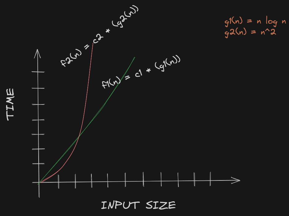
we can see that f2(n) (which is the running time of B's code) takes significantly longer time to complete than f1(n) (which is the running time of A's code) when the input size grows large enough. which brings me to my final point:

When we are dealing with input sizes large enough to make only the order of growth our concern, we are studying asymptotic analysis of algorithms

Asymptotic notations

A knowledge of asymptotic notations becomes a tool when we want to give an estimate of the running time of our algorithms. this provides us a way of predicting the behavior of an algorithm in terms of time efficiency when tested against any range of input.

Going by our definition of time complexity, it's safe to say that asymptotic notations lets us analyze the time complexity of algorithms

• Ω(g(n)) (reads "omega-of-..") - this is used to to bound an algorithm's running time from below.

• Θ(g(n)) (reads "theta-of-..") - this is used to provide the exact bound of the running time of an algorithm. It is the closest estimation we can get of an algorithm's running time. Additionally, if you can deduce that the running time of an algorithm is both O(g(n)) and Ω(g(n)), then, the running time of the algorithm is Θ(g(n)). To further explain this, let's think of it as an inequality with :

     O -> >=
     Ω -> <=
     and,
     Θ -> =
  

  and two values x and y as operands of this inequality then:

  x >= y and x <= y implies x = y

• O(g(n)) (reads "big-oh-of-..") - this is used to give an upper bound to the running time of an algorithm.

for this explanation, let's re-use the running times of A and B's algorithms (f1(n) and f2(n) respectively) as an analogy. Let's say in the implementation of B's algorithm, the input does not need to be sorted if it's already a sorted sequence but A's algorithm, although fast, does not have the ability to check if the sequence is already sorted. Consequently, B's algorithm seems to take N (only needs to look into a sequence of size N once) steps in this special case while A's algorithm always takes N log N steps no matter what.

Since B's algorithm now grows at a linear rate if the array is already sorted, let's make a little change to our previous graph:

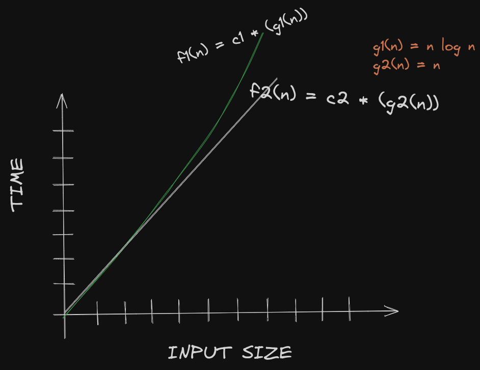
In this special case, we can see that the curve of A's running time goes above B's running time as the input size grows.

This special case is known as the best case. The best case of the running time of an algorithm is when the algorithm is supposed to do less work than usual. In the case of both A and B's algorithms, the best case is when the input is already a sorted sequence. The worst case on the other hand, is when the algorithm is expected to do the most work.

A common misconception most programmers have is thinking that "case" is the same thing as the "bound" which have we have seen, is different. Now with the newly obtained information, let's use the three notations defined earlier to provide the time complexities of A and B's algorithms

A's running time estimation (or time complexity)

• Ω(nlogn) : since we already know that the running time of A's algorithm doesn't get any lower than N log N (even in the best case), we can say that N log N is a lower bound estimation on the running time of A's algorithm. Hence, f1(n) is :

f1(n) = Ω(nlogn)                   ===>( 0.1 )

• O(nlogn): remember that this provides an upper bound estimation on the running time of an algorithm. Therefore, since the running time of A's algorithm doesn't go beyond N log N (even in the worst case), we can say that N log N is an upper bound estimation on the running time of A's algorithm. Hence, f1(n) is given by:

  f1(n) = O(nlogn)                 ====>( 0.2 )

• Θ(nlogn): because the lower bound in (0.1) and the upper bound in (0.2) have the same value, we can say that this is an exact bound estimation on the running time of A's algorithm. Hence, f1(n) is :

f1(n) = Θ(nlogn)

B's running time estimation (or time complexity)

• Ω(n) : since we already know that the running time of B's algorithm doesn't get any lower than N (even in the best case), we can say that N is a lower bound estimation on the running time of A's algorithm. Hence, f2(n) is denoted by:

  f2(n) = Ω(n)                   ===>( 1.1 )
  

• O(n^2): recall that this provides an upper bound estimation on the running time of an algorithm. Therefore, since the running time of B's algorithm doesn't go beyond N^2 (even in the worst case), we can say that N^2 is an upper bound estimation on the running time of B's algorithm. Hence, f2(n) is denoted by:

f2(n) = O(n^2)                 ====>( 1.2 )

• Θ(?): This is the interesting part because the upper bound of B's algorithm is not the same as the lower bound of B's algorithm. Therefore, we cannot find the exact bound on B's algorithm for all input sizes and cases

Sometimes, "It Depends" Is The Right Answer

Our issue with B's algorithm is that we can only deduce it's upper and lower bounds but not it's exact bound. And that is totally fine because we can use any of the bounds we have already obtained. But which one is a better choice comes down to what we need them for. Sometimes, you just want to know the least amount of time an algorithm can take but usually, we as programmers want look at it from above (i.e the most amount of time it can take) because this way, we can expect our algorithm not to take longer than that time - which is more useful in real world applications. And that is why the O notation, aka "big-Oh", is the most popular kid in the block, since it's always available and predictable.

But would we be wrong if we said B's algorithm takes both Θ(n^2) and Θ(n)?

As you might have guessed, it depends on the context: To help you understand better, let's first make statements that will be considered false. these set of statements,
a. B's algorithm is Θ(n^2) in the best case

b. B's algorithm is Θ(n) in the worst case

c. B's algorithm is Ω(n^2) in the best case

are false because
a. we saw that B's algorithm had a better running time in the best case - which is N. And

b. It took way more that N (i.e, N^2) to run when it had the most work to do (let's assume that this is when the input sequence is sorted in the opposite order).

c. this is like saying "it took B's algorithm at least N^2 seconds to run" in the best case which you should already know is false if you read the first reason

but these other statements,
a. B's algorithm is O(n^2) in the worst case

b. B's algorithm is Ω(n^2) in the worst case

c. B's algorithm is Θ(n^2) in the worst case (from the definition of Θ(g(n)) we provided earlier)

d. B's algorithm is Ω(n) in the best case

e. B's algorithm is O(n) in the best case

f. B's algorithm is Θ(n) in the best case (from the definition of Θ(g(n)) we provided earlier)

are in fact true.

That's it guys! I hope you found this blog useful. I'm Daniel, I share stuff about software engineering and i make some cool projects on github